Threat Hunting with Jupyter Notebooks – Part 1: Connect to Elasticsearch

So today I wanted to talk about threat hunting with Jupyter Notebooks. I will cover what a Jupyter Notebook is. I will also cover what Elasticsearch is, this will be where the data we analyze is located. We will look at how to connect to our Elasticsearch instance, get it formatted in a way that looks good and do a couple basic queries. In later posts on this topic we will go more in depth in the data we query for hunting purposes.

What is a Jupyter Notebook? According to the official documentation, “The notebook extends the console-based approach to interactive computing in a qualitatively new direction, providing a web-based application suitable for capturing the whole computation process: developing, documenting, and executing code, as well as communicating the results. The Jupyter notebook combines two components:

A web application: a browser-based tool for interactive authoring of documents which combine explanatory text, mathematics, computations and their rich media output.

Notebook documents: a representation of all content visible in the web application, including inputs and outputs of the computations, explanatory text, mathematics, images, and rich media representations of objects.” 

So in effect, it allows you to run your code and see immediate results in your browser. It is really effective, in my opinion, at documenting your hunts, because as you run your queries and results are returned they are saved in your notebook. This can be beneficial for your junior analysts as they can look at notebooks that have been prepared by more senior analysts and get an idea of their workflow as they approach a hunt.

What is Elasticseach? According to their official site, “Elasticsearch is a distributed, open source search and analytics engine for all types of data, including textual, numerical, geospatial, structured, and unstructured. Elasticsearch is built on Apache Lucene and was first released in 2010 by Elasticsearch N.V. (now known as Elastic). Known for its simple REST APIs, distributed nature, speed, and scalability, Elasticsearch is the central component of the Elastic Stack, a set of open source tools for data ingestion, enrichment, storage, analysis, and visualization. Commonly referred to as the ELK Stack (after Elasticsearch, Logstash, and Kibana), the Elastic Stack now includes a rich collection of lightweight shipping agents known as Beats for sending data to Elasticsearch.”

Well that sounds like the perfect place for me to store my data in order to search through it!

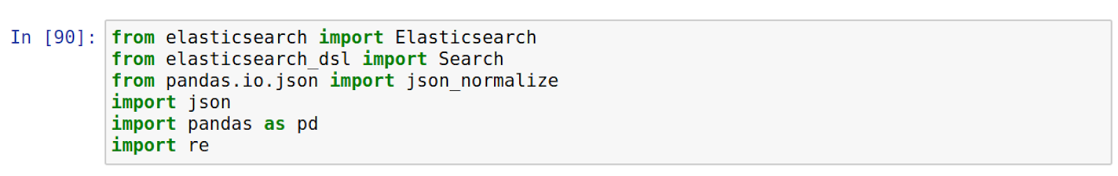
Now that we understand what a Jupyter Notebook and Elasticsearch is, let’s talk about some of the Python libraries we will need to connect and search through our Elasticsearch data. So in this series I will be using Python. First thing I recommend doing on your analyst machine is to download the Anaconda distribution. Anaconda will install Jupyter Notebook and most of the Python data science libraries we will need. The only other libraries that need to be installed are elasticsearch and elasticsearch-dsl, which can be done through pip.

Let’s start by spinning up our Jupyter Notebook server by navigating to: /root/anaconda3/bin, then ./jupyter-notebook. Then from there open your favorite browser and go to localhost:8888. Create a notebook by selecting new and then Python3.

Next we need to import our libraries. Below is a screenshot.

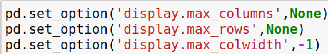
We will now set some options which will allow us to view all of our data. Jupyter will by default crop out some of your data. For example if you have a ton of columns in your DataFrame, Elasticsearch will crop some out, which you will know by seeing “…”. 

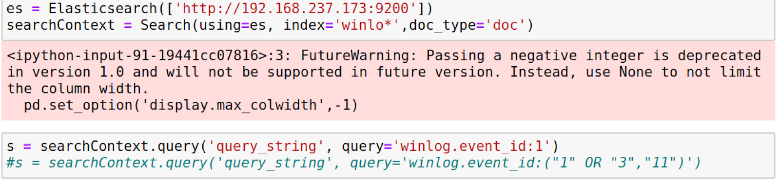
Now that we have our libraries imported and set our options, we need to connect to our Elasticsearch, set a search context and set a query. In this instance I’m connecting to my Elasticsearch instance at 192.168.237.173:9200. I will be looking at my winlogbeat index and looking only at Sysmon event ID 1, which are process creates. 

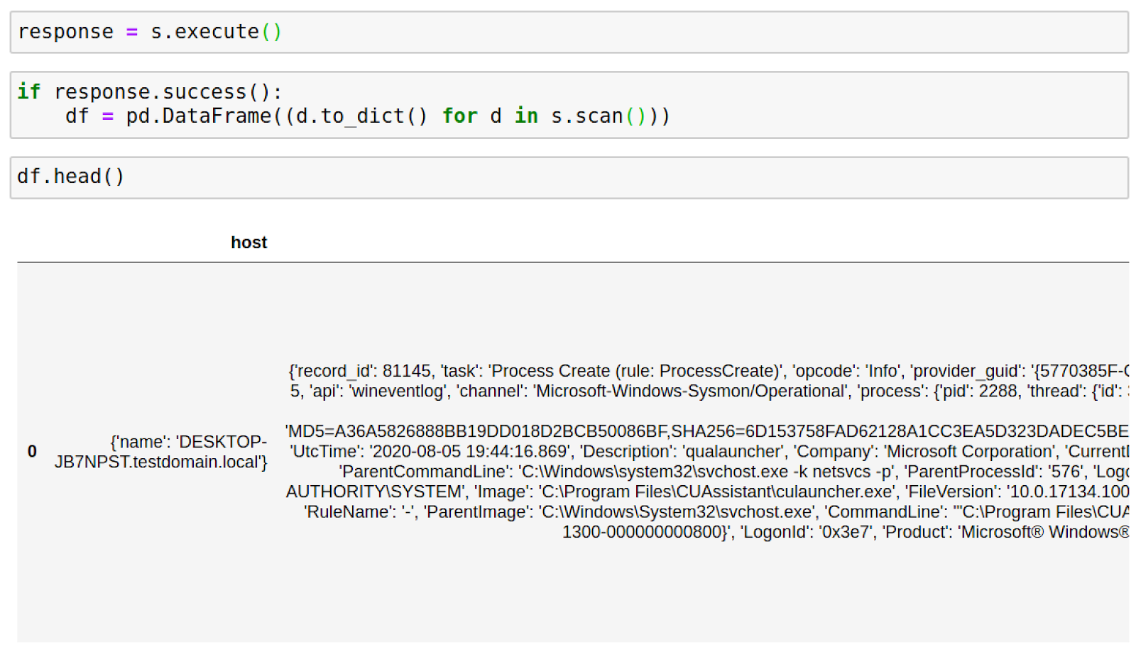
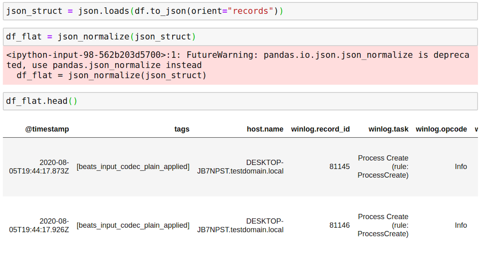
We now do a “for loop” through our response variable return only successful requests from our Elasticsearch server and store them in a DataFrame of nested dictionaries, which we will have to flatten to make it look good. We will do a quick head() on our data to make sure we have some.

Now we will convert our DataFrame back to json and then use json_normalize to flatten out our data and do a head() to ensure our data was formatted properly.

Excellent! We have our properly formatted DataFrame of our Sysmon event ID 1’s now, so let’s do a basic query so you can see the power of the pandas library. 

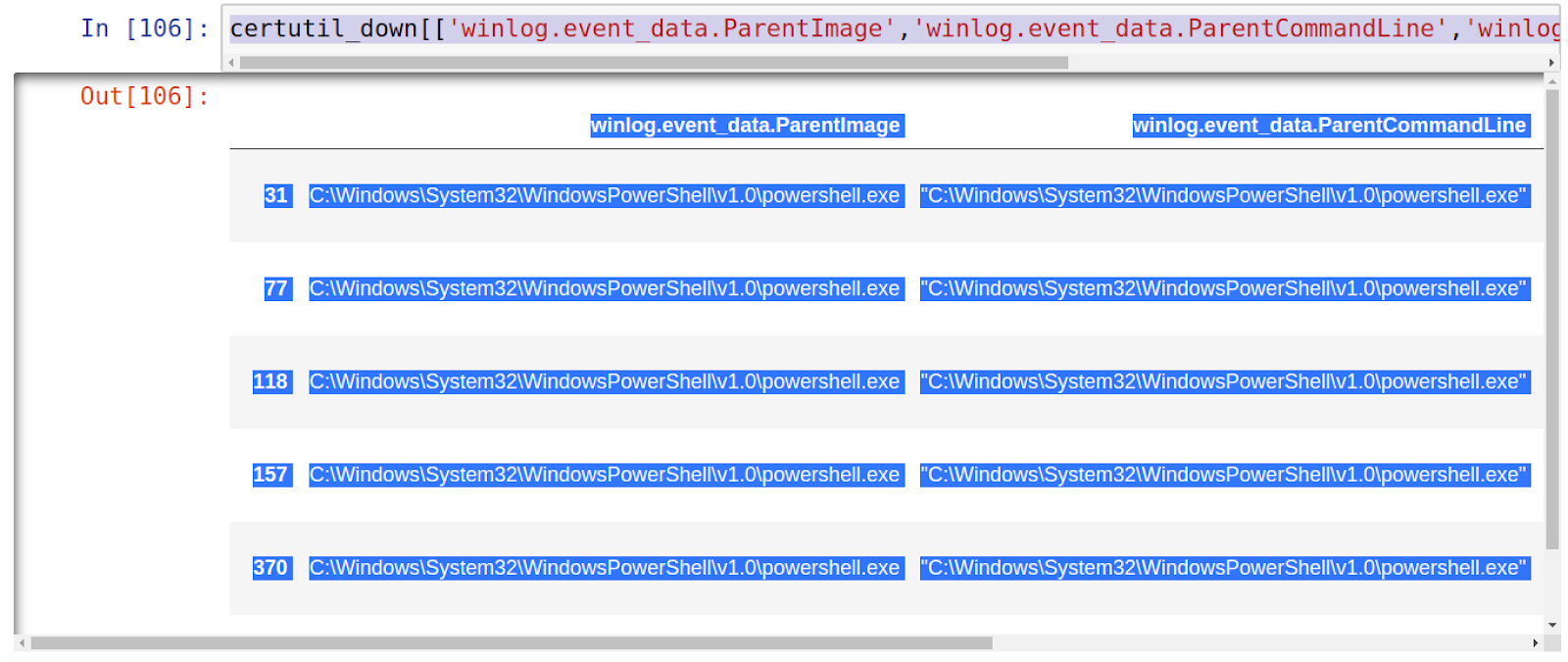
For my hunt hypothesis I am proposing attackers in my environment are running PowerShell and certutil.exe to download files from their Command and Control (C2) server. I create a variable named certutil_down: 

certutil_down = df_flat[(df_flat[“winlog.event_data.Image”].str.contains(“certutil.exe”,flags=re.IGNORECASE) == True) & (df_flat[“winlog.event_data.ParentImage”].str.contains(“powershell.exe”,flags=re.IGNORECASE) == True)]

This query is looking in my normalized DataFrame and I’m using regular expression ignoring case looking for a Parent Process of PowerShell running a Child Process of certutil.

Since this will also return some data I don’t want I will filter it down to only return the Image, ParentImage, CommandLine and Parent CommandLine with this query:

certutil_down[[‘winlog.event_data.ParentImage’,’winlog.event_data.ParentCommandLine’,’winlog.event_data.Image’,’winlog.event_data.CommandLine’]]

So there you have it, I hope this has been useful at showing some of the power of using Jupyter, Elasticsearch and Python. Until next time…

Happy Hunting,

Marcus

References:

1. https://jupyter.org/
2. https://jupyter-notebook.readthedocs.io/en/stable/notebook.html
3. https://www.elastic.co/what-is/elasticsearch
4. https://www.anaconda.com/products/individual